
19: Multiplication and Division Circuits


Though still relatively straightforward, multiplication and division circuits are more complicated than addition and subtraction circuits. Multiplication with two numbers, for example, is really nothing more than an addition performed some number of times: take, for instance, the numbers 45 and 32 (45* 32=1440).
This computation is just 32+32+32+32+32+…+32, 45 times. Alternatively, 45+45+45+…+45 gives the same result in 32 steps. As we all know, these exact computations are superfluous: We don’t need all intermediate values. If we did multiplication like this, it would take a minimum of 32 passes through the addition circuit before getting a final answer. This would take a long time.
To solve this problem efficiently, let’s take inspiration from the previous post and, like with our final subtractor, recall what we’ve learned in primary school. Specifically, we will need to use what I back then called “schriftliches multiplizieren”, i.e., long multiplication. If we were to multiply two numbers on paper, we would calculate 40*30 + 40*2 + 5*30 + 5*2, which in our childish’s eyes, was doable. We’d multiply two numbers together, then add the appropriate number of zeros at the end.
Easy enough, but this algorithm has too high space and time complexity. If the number of digits in each number is n, then the number of passes through the addition circuit will result in an O(n²) time complexity (because you multiply each digit with every other digit) as well as in space complexity (for each of these calculations you need to save the number). You could reduce space complexity to O(1) (constant space) by adding the multiplied numbers together after every calculation. But the important property is the O(n²) time complexity, which will cause significant problems when we multiply two large numbers together. So while this is a better solution than our previous one, it isn’t a long-term solution for general-purpose computers.
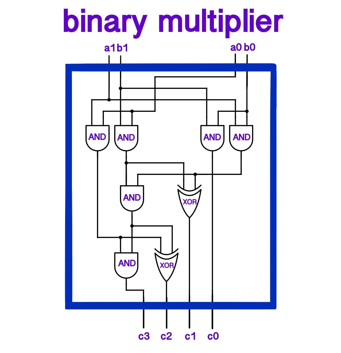
A better solution is to use a separate circuit for multiplication, just as we’ve done with addition & subtraction. We start by extending vocabulary: the Least Significant Bit (LSB), in a binary representation of a number, is the one with the smallest value (we assume that it is the right-most bit). This bit is the one that defines whether a number is odd or even. On the flip side, we also have the Most Significant Bit (MSB).
The LSB will be easiest to compute (a_0, b_0, defining odd or even. r_0 will be the LSB result), as it only depends on the first digit of both numbers. We know an even number multiplied by any other number is always even. The only time two numbers multiplied together give an odd number is when both numbers are odd. Therefore, for the last digit of our result, we AND the two last bits of our two numbers to get the last bit of the result for the multiplication.
To compute the next digit, we put the a_0 and b_0 values and those of the next digit (a_1, b_1) into a full adder (accepting a carry from the LSB computation), which gives a (partial) result for the second bit. Like in long division, every bit needs to be “multiplied” with every other, so a first row of adders will only compute an intermediary result. We must extend this circuit to have another row of full adders that computes the multiplications of more digits. With this new row, we are able to compute the final r_1. This leaves us, however, with all the other r_n values.
The full multiplication, then, consists of a row for every bit of the possible result, which means that our circuit thus results in a parallelogram known as a Wallace tree. Each “point” in this shape makes up a full adder, with the exception of the half adder we used to compute r_0. You can verify the exact mechanism yourself and that the circuit really does multiply two numbers together. This method takes O(n²) computations, like long division.
In general, the multiplication circuit isn’t used commercially for commercial computers. The issue with this circuit is that it is fairly large, especially if you want to use ripple look-ahead adders. But even without, you are using 18 transistors per full adder, which gives us around 64*64*18=74’000 transistors. A better multiplier design, known as Dadda Multipliers, results in fewer needed transistors to multiply two numbers together, around (64/2)²*20~= 20 ‘000 transistors).
So far, we’ve been multiplying integers. But multiplication with fractions works in a very similar way. A computer needs to remember where to place the radix point, the little dot that specifies from which number onward the digits define a fraction. Because this radix point “floats” in between the digits and even changes its position (when multiplying two of them, for example), any number that has a fractional component is known as a floating point number (as opposed to fixed-point numbers), which usually take up the maximum amount of bits that is possible for any architecture.
Multiplication of negative numbers can also be handled. The simplest solution is to note the resulting sign of the computation and assume that all inputted numbers are positive. However, one can also apply two’s complement and other tricks in order to get the multiplier to achieve multiplication of a negative number, although which exact multiplication method one uses depends on what the hardware needs to achieve.
While this result is satisfying, this is not how multiplication is done on commercial chips, like the ones on your computer. Even though these circuits can compute values very quickly, chip manufacturers need to consider the physical space they use up. Tens of thousands of transistors use a lot of space and energy, so manufacturers opt not to build a dedicated multiplication circuit. One would also be unable to multiply numbers with results that are larger than 2^64.
The solution to these problems is to use algorithms that can multiply any two arbitrarily large numbers together. One such algorithm is Karastuba’s algorithm, which uses the clever insight that multiplication can be done in a small number of additions. This algorithm is central to multiplication, although new methods were invented for larger and larger numbers that worked better in practice. The Toom-Cook algorithm builds on Karatsuba’s algorithm and is one of the best multiplication algorithms to date. However, in the special case that two numbers are in the range of 15000–70000 digits long (!!), the (to me, mind-blowing) Schönhage-Strassen algorithm performs better.
What the best way to do multiplication exactly is, is a question for the academics. With this, we leave multiplication behind and move on to digital division.
While multiplying two integers, any two integers, we know that it results in another integer. But dividing two integers together can result in floating point numbers, which can be expensive to compute if one is trying to account for every bit of memory used in, say memory restricted circuits. For this reason, there is a difference in how much space is needed when dividing two numbers either through “normal” division, division to the nearest integer, or division with remainder.
It is because of this that multiple division algorithms, as well as circuits, have been invented that do division in particular ways. Long division, as most of us did in school, is a relatively expensive procedure while also getting an exact-as-possible number as a result. But often, this isn’t needed in certain technologies, where an integer value is exact enough. Some technologies only require the division to the nearest integer.
One example of a dedicated circuit to do precise division is one given on StackExchange, although division is usually done using algorithms. One can verify that it works by plugging in some binary numbers and seeing the circuit through, though this is a lot of work to do as a casual reader or writer. I haven’t verified that the circuit actually works; I found it online here and figured I’d blindly show you this caveat. I think (?) it works (???). For what it’s worth, I trust the super nerds on the internet that the given solution is correct.
When it comes to doing division using algorithms, the length of an article like this (and its “light” reading style) won’t do them justice. Two algorithms can divide effectively: The first is known as the Newton method, which is an algorithm that tries to estimate the result with higher and higher levels of specificity. The other is known as the Goldschmidt method, which tries to divide numbers using multiplication, concatenation, and addition. There is also complement division.
With this, we conclude the first step in building a computer by having rounded off arithmetic with a basic overview of multiplication and division. Beyond these common operations, there are plenty more operations that one can perform on bits that do not include these and are necessary for a multitude of software applications.
Inevitably, we now turn our attention to operations on memory, registers, and bits in general.